
Ask any PhD students and they will tell you that literature review is a daunting task. Sifting through mountains of papers to find the specific information that you need is no easy feat, especially there are often conflicting information, and worse, abstracts that looks promising but nothing of interest actually offer in the full-text. There is good reason why literature survey forms a significant part of the PhD thesis – you literally spend at least a month on it! Is there a better way?
With the increasing capability of natural language processing, there is scope to automate some part of the literature review. Wouldn’t it be nice if a computer can do the sifting work and identify the articles that are actually important? In this and the next two blogs, I will be going through how one can utilise natural language processing to extract important papers for review.
The example presented here is part of a Kaggle’s Open Challenge – the CORD-19 Open Research Dataset challenge. The idea of the challenge is that with the rapid increase of the number of articles published about COVID-19, medical experts and researchers is finding it hard to find relevant information in a timely manner, especially when they have to race against the clock to find treatment for a dying patient or to find a cure as soon as possible to reduce casualties. So the Allen Institute asked the Kaggle community in this open challenge for possible solutions to this problem. As a part of the challenge, they provided the full text of a large number of articles in json format, as well as the metadata for these articles, including the DOI, titles, abstract, and authors in a csv format. Loading this csv into python using pandas yield the following:

The most obvious way to work on this data is to first only consider the metadata and try to narrow down to the relevant articles using just the title and abstract. Since in most cases, the title contains the most summarised information compared to an abstract, I am going to take a three tier approach. First, I will separate the articles into topics by preforming topic modelling on the titles. This is followed by a clustering analysis on the abstract of articles that falls into the relevant topics to select the most relevant abstract cluster. Finally, the full text of this abstract cluster can be pulled out and summarized using text summarization. This first blog will consider the first step – topic modelling.
Text Preprocessing
Similar to normal data, most text needs to be cleaned before applying natural language processing techniques. To make a data analogy, a block of text in a large text document or a sentence in a paragraph is like a row in a dataframe, and each word is the data entry of that row. We need to make sure that these words are all in the same form and is understandable to a machine in order to perform NLP. For example, a key operation in text preprocessing is turning all letters into lower case. That’s because the computer will consider two words, such as “Hello” and “hello” as different as they are represented differently in the computer. In order for the computer to recognise that they are the same, the best way is to turn everything into lower case. Some other important and common operations include removing punctuation and removing numbers. These can be done easily using regular expressions:
import re
import string

def text_cleaner(text):
    text = str(text).lower()
    text = re.sub('[%s]' % re.escape(string.punctuation), '', text)
    text = re.sub('[0-9]', '', text)

    return text

text_df.title = text_df.title.apply(lambda x: text_cleaner(x))
Another common operation that may or may not be helpful is stemming or lemmatizing. Consider words such as “eat” and “eating”. In most cases, they have very similar meaning. How can we let the computer know to consider them as the same words? One way is to use stemming, which essentially stem the words into a shorter form by removing common suffixes such as “ing”, “tion” or “s”. In the above cases, stemming would reduce “eating” to “eat”. How about “eat” and “ate”? Stemming would not be able to do anything in this case. What we need is lemmatizing, which reduces a word to its lemma, or dictionary form. Lemmatizing “ate” would yield eat, and lemmatizing “is”, “was”, “are” and “were” would all yield “be”. Stemming and Lemmatizing can be done using Python’s NLTK package. Here, we will use lemmatization on the title data:
from nltk.tokenize import word_tokenize
from nltk.stem import WordNetLemmatizer

#combine the different "virus" forms and combine the term "severe acute respiratory syndrome" into sars"

text_df.title = text_df.title.apply(lambda x:x.replace("severe acute respiratory syndrome", "sars"))
text_df.title = text_df.title.apply(lambda x:re.sub('viral|viruses', 'virus', x))


wordnet_lemmatizer = WordNetLemmatizer()
lemma = WordNetLemmatizer()
text_df['Tokens'] = text_df.title.apply(lambda x: word_tokenize(x))
text_df.Tokens = text_df.Tokens.apply(lambda x: " ".join([lemma.lemmatize(item) for item in x]))
Note additional processing was performed on some keywords that lemmatizer was not able to pick up, such as “virus” vs “viruses”, and “severe acute respiratory syndrome” vs its acronym.
Word Tokenization and Bag of Words
It can been seen in the script above that a word tokenizer was applied. Tokenizing is a fancy word for breaking up a sentence into individual words. This simple action may seem intuitive to us, but is important for the computer to recognise that each word or token has a meaning, and not trying to break it down further. Again, one can use NLTK to break a piece of text into tokens, as above, before further processing.
We can now take a look a random title before and after processing to see the difference they have:


The visible difference is the removal of punctuation and numbers, as well as everything being in lower case. It is also now in a tokenised form, ready for NLP techniques to be applied.
The basis of NLP is trying to use computer to extract meaning from text. One of the simplest ways is to simply look at what words are in the text and to see which words appears the most frequently to tell what the text is above. This is called the bag-of-words, i.e you are treating the text or paragraph as a mixed-bag of vocabularies. The advantage of this technique is that it is simple and easy to produce. The disadvantage of this technique is the loss of information in the arrangement of words or context, which often determines the meaning of a particular word. Nevertheless, the bag-of-words technique works quite well, and this is what we will be doing here.
To create the bag-of-words, we form a matrix where the columns corresponds to each word and the rows corresponds to each document of interest, e.g a sentence, or in this particular case, the title of each article. The element of the matrix then corresponds to the frequency of each word in that particular document of interest. This matrix is called the document-term matrix (DTM). The DTM can be obtained using CountVectorizer() in the scikit-learn package:
from sklearn.feature_extraction.text import CountVectorizer

cv2 = CountVectorizer()
text_cv_stemed = cv2.fit_transform(text_df.Tokens)
dtm = pd.DataFrame(text_cv_stemed.toarray(), columns = cv2.get_feature_names())
top_words = dtm.sum(axis = 0).sort_values(ascending = False)
print(top_words[0:10])
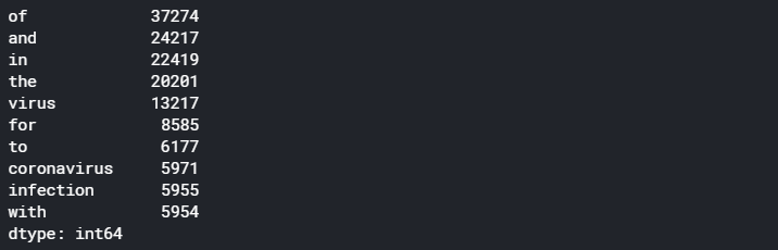
Here, we can see the major problem of a naive word frequency approach – it is dominated by common words such as “of”, “and”, “the”, which offers no information on what the document is about. We need to remove these common terms, via what is known as the stop-words. Stop-words is a list of words which we want to remove in a bag-of-words, and most tokenization methods provides a native list of stop-words that would include most common words in the English language, such as “is”, “are”, “and”, “the”, etc. Many methods also provide ways to add in additional words in the stop-words list so that user can exclude words that are common to most of the documents of interest, and therefore offers no additional information. In our case here, we are also going to remove “virus”, “study” and “chapter” which seems to be appearing a lot but offer no extra information on what the document is above (virus is removed as by default, a lot of the articles will have virus as a keyword since this is a database relating to a virus):
from sklearn.feature_extraction import text
from nltk.corpus import stopwords

stop_words = text.ENGLISH_STOP_WORDS.union(["chapter","study","virus"])
cv2 = CountVectorizer(stop_words = stop_words)
text_cv_stemed = cv2.fit_transform(text_df.Tokens)
dtm = pd.DataFrame(text_cv_stemed.toarray(), columns = cv2.get_feature_names())
top_words = dtm.sum(axis = 0).sort_values(ascending = False)
print(top_words[0:10])
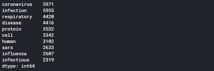
We can see that out of the 40k+ titles, some of the most common terms include “Coronavirus”, “respiratory”, and “disease”. The bag-of-word technique has done a reasonable job in extracting the keywords of the titles for the articles of interest and gives us a general idea of what all these articles are about.
Next, we want to look at how the titles can be separated into different topics using this bag-of-words or DTM that we have just generated. To do this, we use Topic Modelling.
What is Topic Modelling?
Topic Modelling is an unsupervised clustering technique that assign different topics to the documents in the training set. It uses the bag-of-words approach and assumes that each document is described by a statistical distribution of topics, and each topic is defined as a statistical distribution of words. Essentially, topic modelling looks at the word frequency of different words in each document, and assumes that documents with a similar word frequency of the same words are of the same topic.
As a simple example, let’s say we have five sentences:
- “I have a cat and I love cats”
- “Cats are carnivorous mammals. Lions and Tigers are also of the cat family”;
- “Both Dogs and Wolfs are Carnivorous. Wolves like to hunt in packs “
- “Banana and Apples are great for making desserts. I love them”
- “Hunter likes to use hunting dogs to help them hunt because of their great sense of smell”
It can be seen quite easily that one may be able to group these sentences into different topics by simply looking at the words used and how frequent they were used. For example, the first and second sentence are about cats – they both have cats occurring twice in the sentences. The third and last sentence have hunt and dog appearing, and therefore can be grouped into a topic, and there is a very weak link between the first and the fourth sentence through the words “I love” and so there could be a topic that would be assigned to both.
Topic modelling seek to do the above automatically. In real situations, with significantly longer documents and larger word base, it would be much harder to assign topics by simply matching exact words and frequencies. This calls for a more statistical approach – something known as Latent Dirichlet Allocation (LDA)
Latent Dirichlet Allocation(LDA)
In LDA, the topics are assume to be “hidden”, i.e. there is assumed a hidden set of topics that generates all of the documents (hence the term latent). It assumes that the probability of the nth document containing words in the mth topic follows the Dirichlet distribution (As this article is more practically focused, I won’t go into details of the Dirichlet distribution here). The LDA algorithm works by first randomly assigning each word in each document into one of the topics, and then for each word in each document, look at the current proportion of all words in the document that are assigned to the topic that the word belongs to, and the current proportion of all documents that are assigned to this topic because of this word. The word’s topic assignment is then updated according to the Dirichlet distribution. This is repeated for all words and all documents for a large number of times until it reaches a steady state.
Despite the complex mathematics and algorithms involved in the LDA, thankfully the python package gensim provides a simple way to do this:
from gensim import matutils, models

#First, the dtm needs to be transposed into a term document matrix, and then into a spare matrix

tdm = dtm.transpose()
sparse_counts = scipy.sparse.csr_matrix(tdm)

#Gensim provide tools to turn the spare matrix into the corpus input needed for the LDA modelling.
corpus = matutils.Sparse2Corpus(sparse_counts)

#One also require a look up table that allow us to refer back to the word from its word-id in the dtm
id2word = dict((v,k) for k, v in cv2.vocabulary_.items())

#Fitting a LDA model simply requires the corpus input, the id2word look up, and specify the number of topics required

lda = models.LdaModel(corpus = corpus, id2word = id2word, num_topics=20,
                                           passes=10,
                                           alpha='auto')

lda.print_topics()
A few things of note. Firstly, the gensim LDA routine takes in a term-document matrix (TDM) instead of the document-term matrix. We therefore need to transpose the DTM output from CountVectorizer. Also, as the TDM is a sparse matrix, we can store it as a scipy sparse matrix object for more efficient calculations. Finally, we require a look up table between the word ID and the actual word which we can obtain from the CountVectorizer.vocabulary_ attribute. All these are then simply put into the LDA model for training.
If we now print the topics obtained by using print_topics(), the following will be displayed:
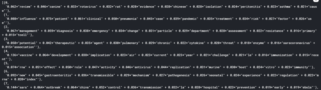
It can be seen that each topics is expressed as the sum of a list of words, weighted by their relative importance in the topic, which is a number from 0 to 1. We can see from the list of topics that in all topics, there is not really a overly dominant word, with the highest importance for each topic falling in the range of around 0.1. This is in fact what usually happen in real life scenario, as it is unlikely that the underlying topics in a complex mix of documents can be described by one or two words alone. Nonetheless, we have successfully performed topic modelling using LDA and have seperated the 40k+ articles into manageable topics.
Optimising the Model
One thing that can be tuned in a topic model is the number of topics. With known documents, we might have some ideas of how many topics there are. However, in most real life scenario such as this one, it would be impossible to know the number of topics to use a priori. We would therefore need to tune the number of topic as a hyperparameter of the LDA model.
In order for tune the number of topics, we need a metric to measure how good a model is. The metric that is commonly used for evaluating topic models is the coherence score. The discussion of what the coherence score actually means is beyond the scope of this blog. However, one could roughly interpret the coherence of a topic model as how semantically similar articles in a topic are to each other. The higher the coherence is, the better the model. Therefore, we can tune the LDA by evaluating the coherence score of models with different number of topics. This is done by invoking the CoherenceModel() in gensim, using the C_v coherence measure.
from gensim.models import CoherenceModel
from gensim import corpora
from matplotlib import pyplot as plt

#The Coherence model uses a corpora.Dictionary object that have both a word2id and id2word lookup table.

d = corpora.Dictionary()
word2id = dict((k, v) for k, v in cv2.vocabulary_.items())
d.id2token = id2word
d.token2id = word2id

#Function to create LDA model and evalute the coherence score for a range of values for the number of #Note that the coherence model needs the original text to calculate the coherence

def calculate_coherence(start, stop, step, corpus, text, id2word, dictionary):
    model_list = []
    coherence = []
    for num_topics in range(start, stop, step):
        lda = models.LdaModel(corpus = corpus, id2word = id2word, num_topics=num_topics, passes=10,alpha='auto')
        model_list.append(lda)
        coherence_model_lda = CoherenceModel(model=lda, texts=text, dictionary=dictionary, coherence='c_v')
        coherence_lda = coherence_model_lda.get_coherence()
        print("Coherence score for ", num_topics, " topics: ", coherence_lda)
        coherence.append(coherence_lda)

    return model_list, coherence

#Create and evaluate models with 10 - 80 topics in steps of 10
model_list, coherence_list = calculate_coherence(10, 90, 10, corpus, text_df.Tokens.apply(lambda x: word_tokenize(x)), id2word, d)


# Plot graph of coherence score as a function of number of topics to look at optimal number of topics.
x = range(10, 90, 10)
plt.plot(x, coherence_list)

plt.title("Coherence Score vs Number of Topics")
plt.xlabel("Number of Topics")
plt.ylabel("Coherence score")
plt.show()
which yields the following:
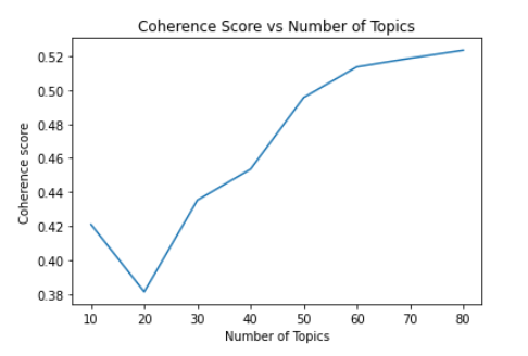
The optimal number of topics is where any further increase in the number of topics does not improve the coherence score. In the graph above, we can see that 60 is a good choice for the number of topics.
Visualising the model
Since the LDA model is a high-dimensional model, it is difficult to visualise the topics and their relation to each other. Fortunately, there is a python package pyLDAvis, which makes use of dimensional reduction for visualising how close each topic is to each other in a LDA model. Let’s try to visualise our model as follows:
# Visualize the topics
pyLDAvis.enable_notebook()
#Taking the 6th model representing 60 topics
vis = pyLDAvis.gensim.prepare(model_list[5], corpus, d)
vis
It may take a while to run, but it produces an interactive graph that let you view the intertopic distance, as well as the word distribution of each topic:
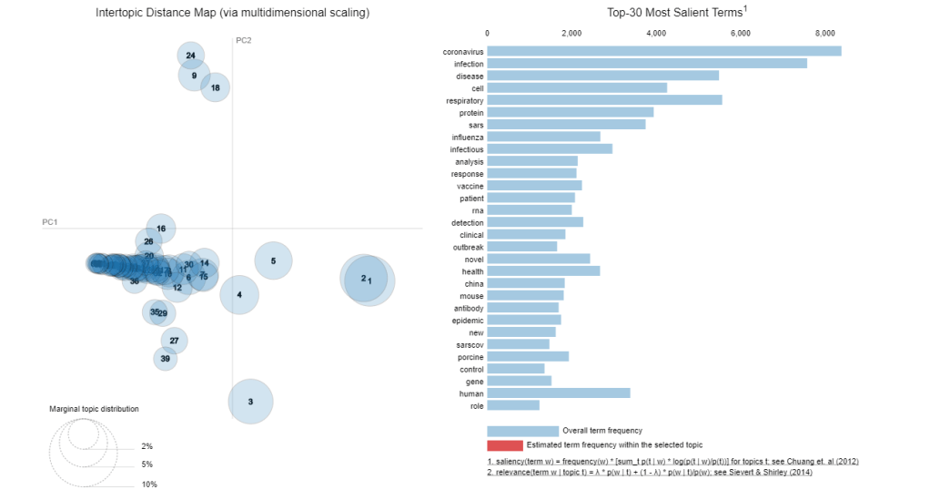
A good topic model would have well spread out models in the 2D principal component space, and that there will be minimal overlap between topics. Of course, that is only in ideal situation. We can see here that there are substantial overlap between the models. with models congregating as a streak across a small part of the 2D space. This indicates that the LDA model didn’t perform particularly well. However, overlap is pretty much expected when we try to reduce 40,000 articles into 60 topics, so the fact that there are quite a few non-overlapping models shows that LDA is at least a promising approach. A possibility of the poor performance is that short sentences such as that occurs in a title is known to perform poorly with LDA (see this paper here for example). Nonetheless, we have successfully applied topic modelling to this large set of articles and this will allows us to narrow our literature search.
Assigning Topics
The final task in topic modelling for our problem at hand is to assign a topic to each of the article using the topic model. One can obtain the topics predicted particular document via the code below:
#Format the title in a form acceptable by the gensim lda model
corpus_dict = Dictionary([text_df.title[0])
corpus = [corpus_dict.doc2bow(words) for words in [text_df.title[0]]
#predict the topic probabilities using the model
vector = model_list[5][corpus]
topic_list = []
for topic in vector:
      print(topic)
Note that the input into the lda model must be in a bag-of-word form, converted using a gensim Dictionary created from the text. If we print the result, we will get something like this:
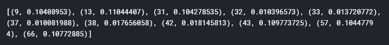
We see the model prediction results in a list of tuples, with the first element the topic number, and the second number a probability or weight of that particular topic. Again, this is the direct visualisation of how a LDA model assumes each document has a distribution of topics and predicts such models and their distribution when a document is passed into the model. Similar to the words in the topic, we see that for most document, there is not one topic that significantly dominate the document, but rather a few equally likely topics with similar probability. For the purpose of separating the articles, let’s take the top three topics to represent each article, and store them into the initial dataframe:
#Store tht top 3 topics, the contribution of the most dominant topic, and the total contribution of the top three topics
topic_list = []
top_score = []
sum_score = []
#lda_mode[corpus] gives the list of topics for each sentence (list of tokens) in the corpus as a list of tuples. We can then decipher that
#and extract out the top three topics and their scores
for i, row in enumerate(model_list[5][corpus]):
    top_topics = sorted(row, key=lambda tup: tup[1], reverse = True)[0:3]
    topic_list.append([tup[0] for tup in top_topics])
    top_score.append(top_topics[0][1])
    sum_score.append(sum([tup[1] for tup in top_topics]))

text_df['topics'] = topic_list
text_df['top_score'] = top_score
text_df['sum_scores'] = sum_score
text_df.head()
With a trained topic model and the predicted topic for each article, we are now ready to go into the next part: a more in-depth clustering study using word vectors. This will be covered in the next blog.
The full version of the code and results presented here can be found here
References:
https://towardsdatascience.com/latent-dirichlet-allocation-lda-9d1cd064ffa2
http://blog.echen.me/2011/08/22/introduction-to-latent-dirichlet-allocation/

One thought on “COVID-19 Literature Review using Natural Language Process – Part #1 Topic Modelling”