In the last blog I have showed how to use topic modelling to seperate a large number of articles into different topics. In this blog, I am going to talk about how to take one step further, and use word vectors and clustering to track down the articles that you really need.
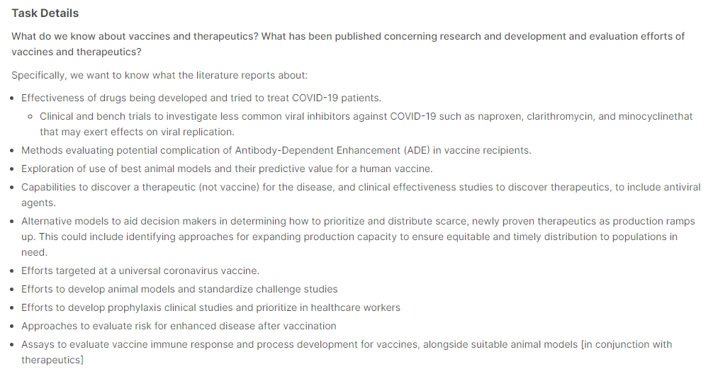
Recall from the last blog that each articles have been assigned three top topics using topic modelling. We will now use this to narrow down the articles that we need. Then, we need to first look at what we are looking for in these articles. The Kaggle Open Challenge specified a range of tasks for the participants to work on. Here, I will be focusing on the task related to Vaccines and Therapeutics for COVID-19, as specified in this page. The task is essentially answer the questions posed on the page:
To select the topics that are relevant to these questions, we can extract out the keywords from these questions using a technique known as term frequency–inverse document frequency, or TF-IDF, and then select the topics which contain these keywords.
TF-IDF
Recall from the last blog, topic modelling is a bag-of-words method – a technique that considers words as individual tokens and uses its frequency of appearance as a key indicator of what a document of text, which is called a corpus, means. TF-IDF also make use of bag-of-words. As the name suggests, it too looks at the frequency of appearance of words in a document (the Term Freqency TF). However, it also looks at the frequency of appearance of the word across all documents, and reduce its weight if appears too often (the Inverse Document Frequency IDF). By applying this counter-weight, TF-IDF is able to filter out common words that appears everywhere and offers no extra information for distinguishing different documents. In its simplest form, the TF of a word is simply the number of times it occurred in one document, scaled by the number of words in the document. For example, in “How much wood could a woodchuck chuck if a woodchuck could chuck wood”, all three words “wood”, “woodchuck” and “chuck” has a TF of 2/13. The IDF on the other hand, is given by log(total number of documents/ number of documents containing the word). For example, if we now have 3 other sentences, all of which contain “wood”, 1 contain “chuck” and none contain “woodchuck”, then the IDF of “wood”, “chuck” and “woodchuck” would be 0, log(4/2) and log(4/1) respectively. The TF-IDF is then simply the product of TF and IDF, which gives 0, 0.046 and 0.093 for “wood”, “chuck” and “woodchuck” respectively (for the first sentence only). The word “woodchuck” can be consider as a word that can better distinguish this sentence from the other sentences, comparing to “wood” and “chuck”.
Python Sci-kit Learn provides a quick implementation of TF-IDF. We will use this to extract out the keywords from our list of sentences (Note that question_list is formed by simply putting the questions above into a list):
from sklearn.feature_extraction.text import TfidfVectorizer
import re
import string
from nltk.tokenize import word_tokenize
from nltk.stem import WordNetLemmatizer

#Put list into a dataframe for easier viewing and manipulation
df_task = pd.DataFrame(question_list, columns = ['tasks'])
df_task.head()

#Define function to clean text
def text_cleaner2(text):
    #Convert to lower case
    text = str(text).lower()
    #Remove punctuations
    text = re.sub('[%s]' % re.escape(string.punctuation), " ", text)
    return text
df_task['tasks'] = df_task.tasks.apply(lambda x:text_cleaner2(x))
df_task.head()

#Create TFIDF model note that min_df was tuned to give optimal output
vectorizer = TfidfVectorizer(min_df=0.08, tokenizer = lambda x: x.split(), sublinear_tf=False, stop_words = "english")
tasks_keywords = vectorizer.fit_transform(df_task.tasks)

#Grab all keywords in the TF-IDF vectorizer
new_dict = vectorizer.vocabulary_
#manually remove useless words and put into a new keyword_list
stop_words = ["use", "tried", "studies", "know", "need", "concerning", "alongside"]
for word in stop_words:
    new_dict.pop(word, None)
keyword_list = list(new_dict.keys())

#Do the same processing as in the previous workbook that was used to form the topic topic titles
#This include the replacement of various keywords, removal of numbers and lemmatization
keyword_list = [x.replace("severe acute respiratory syndrome", "sars") for x in keyword_list]
keyword_list = [re.sub('viral|viruses', 'virus', x) for x in keyword_list]
keyword_list = [re.sub('[0-9]', '', x) for x in keyword_list]
wordnet_lemmatizer = WordNetLemmatizer()
lemma = WordNetLemmatizer()
keyword_list = [lemma.lemmatize(x) for x in keyword_list]

print(keyword_list)
Some important things to note here. Firstly, since we are trying to couple the keywords to the topic model that we have, all of the pre-processing that was used during topic modelling must also be used here. This includes lemmatization and the special cases for “SARS” and “Virus”. However, the order of which these are performed can be tuned. In this case here, lemmatization and number removal are done after the TF-IDF to gain a better set keywords. Printing the keywords, we have the following:
['vaccine', 'therapeutic', 'published', 'research', 'development', 'evaluation', 'effort', 'effectiveness', 'drug', 'developed', 'treat', 'covid', 'patient', 'clinical', 'bench', 'trial', 'investigate', 'common', 'virus', 'inhibitor', 'naproxen', 'clarithromycin', 'minocycline', 'exert', 'effect', 'replication', 'method', 'evaluating', 'potential', 'complication', 'antibody', 'dependent', 'enhancement', 'ade', 'vaccine', 'recipient', 'exploration', 'best', 'animal', 'model', 'predictive', 'value', 'human', 'capability', 'discover', 'therapeutic', 'disease', 'include', 'antivirus', 'agent', 'alternative', 'aid', 'decision', 'maker', 'determining', 'prioritize', 'distribute', 'scarce', 'newly', 'proven', 'production', 'ramp', 'identifying', 'approach', 'expanding', 'capacity', 'ensure', 'equitable', 'timely', 'distribution', 'population', 'targeted', 'universal', 'coronavirus', 'develop', 'standardize', 'challenge', 'prophylaxis', 'healthcare', 'worker', 'evaluate', 'risk', 'enhanced', 'vaccination', 'assay', 'immune', 'response', 'process', 'suitable', 'conjunction']Using these keywords, we can go through and select topics which contains these keywords, and then articles that belong to these topics. Note that if a keyword is not seen in any topics in the topic model, it would throw an error, and so one need to catch such exceptions. Finally, it turns out that name of drugs such as ‘naproxen’, ‘clarithromycin’ and ‘minocycline’ are not present in any topics, so I have manually added ‘antiinflammatory’ and ‘antibiotics’ which is the family of drugs that these drugs belongs to:
from gensim.corpora.dictionary import Dictionary

word2id = word_key.token2id
new_topic_list = []
#Initial test shows that two important keywords, naproxen and minocycline are not in the topic keywords
#Since these are antiinflammatory and antibiotics respectively, I have decided to manually add these keywords into the keyword_list
keyword_list.append('antiinflammatory')
keyword_list.append('antibiotic')
for word in keyword_list:
    try:
        word_id = word2id[word]
        topics = topic_model.get_term_topics(word_id, minimum_probability=None)
        for topic in topics:
            new_topic_list.append(topic[0])
    except:
        print(word + " not in topic words")

new_topic_list = list(set(new_topic_list))
Extracting articles that have all three top topics belonging to this new topic list, we find that the number of articles is reduced from 50k to about 10k, i.e 1/5. This is a good reduction and so we are now ready to look at the abstract of these selected articles in depth.
Problems with Bag-of-Words
The bag-of-words method, while quick, simple and useful, ignores the context of a word, which often provides additional information about the document. Consider the following example. Suppose we have the following sentences: “I am going to three banks today to try to get a loan.”; “Usually there are plenty of vegetation along river banks”; “The plane banks towards the airport.” In all three cases, the word “banks” appeared, yet all three have different meanings. Simply looking at the appearance of the word “banks” as a bag-of-word method would is not going to yield a correct topic or meaning for these sentences. What is needed is a technique that takes the context of a word into account. One popular method to do this is the concept of word vectors.
What are Word Vectors?
As the name suggests, word vectors attempts to encode words into multidimensional vectors. The key though is that we want to have these vectors in a way that the distance between words with similar meanings are closer than words with different meanings. For example, we want the word vector for “finance”, “money” and “loan” to be close to each other and to the word “bank” when it is in the first sentence. At the same time, we would want the words “river”, “beach” and the word “bank” in the second sentence to be close to each other but far away from the first set of words. To encode word meaning similarities, one would inevitably have to make use of the position of a word within a sentence. Just like you can infer the meaning of a word that you don’t know by looking at how it is used in a sentence, a computer can potentially identify the similarity of words by looking at words either side of the word of interest.
Word2Vec and Skip-gram
An algorithm that is commonly used for creating word vectors that is implemented by the python gensim package is the Word2Vec algorithm. In the Word2Vec algorithm, each word in a document (the focus word) is considered to be surrounded by a window of n context words. Base on optimising the cosine similarities between the vector representation of the focus word and vector representation of its context words over the whole document, the word vectors for each word are obtained. The relationship of focus words and its context words is visualised below (for a window size of 2):

There are two different ways to optimise a Word2Vec model. In the more intuitive continuous bags of word (CBOW) algorithm, the model optimises the prediction of a focus word given context words. This is similar to the fill in the blank type questions that school kids need to do for their English classes – given a set of context words on either side of the blank, fill in the blank with an appropriate word. For example, “I was at Bondi ____ building sand castles.” The CBOW seeks to predict the focus word given the context words. On the other hand, the Skip-gram algorithm do this in the opposite direction: given a focus word, make a prediction of the context words. This is equivalent to a fill in the blanks question with the following sentence: “____ ____ ____ ____ beach ____ ____ ____”. While this is less intuitive, it turns out that the Skip-gram model actually performs better and hence it is the more popular model to be implemented.
Getting slightly mathematical here, in the skip-gram model, each word has a corresponding focus vector f and a corresponding context vector c, representing when the word is considered as a focus word or context word respectively. The vectors are trained in such a way for two words a and b, the softmax of the dot product afT.bc gives the probability that b is a context word for focus word a, i.e.
P(b|a) = Softmax(afT.bc)
Since we have the ground truth represented by the one hot encoded context words for each focus word, a neural network can be used to trained the word vectors to minimise the overall log-loss of Softmax(afT.bc) for all focus-context word pairs a,b.
Fortunately, we do not have to build this model from scratch. Gensim provides a Word2Vec wrapper to allow a Word2Vec model to be trained and word vectors generated for a document input. I will show you how this is done using the COVID-19 literature dataset.
First, similar to before, we need to clean the abstract first. In particular, almost all abstract entries contacts the word “Abstract” which need to be removed:
from gensim.parsing.preprocessing import remove_stopwords
from nltk.tokenize import word_tokenize
from nltk.stem import WordNetLemmatizer
import re
import string

#Function to clean up abstract
def abstract_cleaner(text):
    #standard preprocessing - lower case and remove punctuation
    text = str(text).lower()
    text = re.sub('[%s]' % re.escape(string.punctuation), "", text)
    #remove other punctuation formats that appears in the abstract
    text = re.sub("’", "", text)
    text = re.sub('“', "", text)
    text = re.sub('”', "", text)
    #remove the word abstract and other stopwords
    text = re.sub("abstract", "", text)
    text = remove_stopwords(text)
    #lemmatize and join back into a sentence
    text = " ".join([lemma.lemmatize(x) for x in word_tokenize(text)])

    return text

#Clean abstract
df_selected['abstract'] = df_selected['abstract'].apply(lambda x: abstract_cleaner(x))
df_selected.head()
Note that there are additional cleaning that was required, namely, there were punctuation symbols that are not in standard format, and therefore cannot be removed with string.punctuation. Stopwords are also removed at this stage.
With the abstracts, because the number of words are much greater compared to titles, we can improve the subsequent word vector model by utilising bigrams. Bigrams are phrases with two words. Phrases such as “Machine Learning” or “Natural Language” are examples bigrams where the two constituent words appearing next to each other in this specific order, offers additional information or even completely new meaning. Therefore, by detecting these as phrases rather than individual words will help reveal more information to the documents we want to analysis. Bigrams can be used via the Phrases and Phraser models within the gensim package.
from gensim.models.phrases import Phrases, Phraser

#Check for bi-grams - first split sentence into tokens
words = [abstract.split() for abstract in df_selected['abstract']]
#Check for phrases, with a phrase needing to appear over 30 times to be counted as a phrase
phrases = Phrases(words, min_count=30, progress_per=10000)
#Form the bigram model
bigram = Phraser(phrases)
#Tokenise the sentences, using both words and bigrams. Tokenised_sentence is the word tokens that we will use to form word vectors
tokenised_sentences = bigram[words]
print(list(tokenised_sentences[0:5]))
Note that the Phraser would turn the sentences into tokens for both single words and bigrams. One can use the Phraser to further look for tri-grams (i.e. 3 worded terms) as well. But we will just stop at bigrams here. One of the tokenised abstract is shown below:
['understanding', 'pathogenesis', 'infectious', 'especially', 'bacterial', 'diarrhea', 'increased', 'dramatically', 'new', 'etiologic_agent', 'mechanism', 'disease', 'known', 'example', 'escherichia_coli', 'serogroup', '0157', 'known', 'cause', 'acute', 'hemorrhagic', 'colitis', 'e_coli', 'serogroups', 'produce', 'shiga', 'toxin', 'recognized', 'etiologic_agent', 'hemolyticuremic', 'syndrome', 'production', 'bacterial', 'diarrhea', 'major', 'facet', 'bacterialmucosal', 'interaction', 'induction', 'intestinal', 'fluid', 'loss', 'enterotoxin', 'bacterialmucosal', 'interaction', 'described', 'stage', '1', 'adherence', 'epithelial_cell', 'microvilli', 'promoted', 'associated', 'pill', '2', 'close', 'adherence', 'enteroadherence', 'usually', 'classic', 'enteropathogenic', 'e_coli', 'mucosal', 'epithelial_cell', 'lacking', 'microvilli', '3', 'mucosal', 'invasion', 'shigella', 'salmonella', 'infection', 'large', 'stride', 'understanding', 'infectious', 'diarrhea', 'likely', 'cloning', 'virulence', 'gene', 'additional', 'hostspecific', 'animal', 'pathogen', 'available', 'study']We can see there are a few bigrams identified, such as “e_coli”, “etiologic_agent”, “epithelial_cell”. As specified when training the model, these bigrams would have occurred more than 30 times throughout all the documents to be counted. With the abstracts tokenised, now we can input this into the Word2Vec model to be trained. There are two important parameters that needs to be specified in gensim’s implementation of Word2Vec(). The first is the window, which specifies how many context words are considered for each focus word. A window size of 2, for example, means that 2 context words before and after the focus word will be considered. The other parameter is the size, which specifies the number of dimension the word vectors will have. Usually a size of a few hundreds will be sufficient. A size of 300 is chosen in our example here. There other other parameters which are learning parameters for the model, such as sample, alpha, min_alpha and negative which can be left as default if wished. One can also specify the number of cores used for training the model to speed up the process.
from gensim.models import Word2Vec
import multiprocessing

#Make use of multiprocessing
cores = multiprocessing.cpu_count() # Count the number of cores in a computer
#Create a word vector model. The number of dimensions chosen for word vector is 300
w2v_model = Word2Vec(window=2,
                     size=300,
                     sample=6e-5,
                     alpha=0.03,
                     min_alpha=0.0007,
                     negative=20,
                     workers=cores-1)

#Build vocab for the model
w2v_model.build_vocab(tokenised_sentences)
#Train model using the tokenised sentences
w2v_model.train(tokenised_sentences, total_examples=w2v_model.corpus_count, epochs=30, report_delay=1)
After the model is trained, each word would now have a word vector associated with it. How can we use or assess whether the model is good or not? We can use two of the most interesting and very powerful features of word vectors – similarity and analogy. The concept of similarity is quite obvious. As one may be able to imagine, words that are similar in meaning would have word vectors close to each other, and therefore the concept of similarity can be applied by looking at the distance between the word vectors, and one would be able to judge whether a model is good by looking at whether a particular word and its synonyms are close to each other.
The concept of analogy is less obvious, and relies on the fact that the dimensions in the vector space actually encodes some meaning in terms of relationship between words. We will use a famous word vector example to illustrate this. Suppose we have the word vectors for “man” and “king”, which are certain distance from each other. Now consider the word “queen”. A Queen is essentially a king but a woman. So one could say that the word vector for “queen” must be the same distance from the word “woman” as the distance between “king” and “man”. Or, to rephrase, we can say that the word vector “queen” is essentially the word vector “king”, taking away the “man” component, but adding the “woman” component. i.e. Vector(Queen) = Vector(King) – Vector(Man) + Vector(Woman). In turns out that this is indeed the case in word vectors, and by using this type of analogy relationships, one can both assess the goodness of the model, as well as potentially use it to obtain information required.
Gensim has the two concept above wrapped into wv.most_similar(), with an identifier positive for getting similarities, and negative for analogy. We can have a look at how well our word vector model for the abstracts is by looking at for example, what terms are the most similar to Covid-19, or look at the analogy of “what word is to Covid-19 as Tamiflu is to influenza”:
print("Top words that are most similar to COVID19:", "\n", w2v_model.wv.most_similar(positive = ["covid19"]))
print("\n")
print("Oseltamivir (Tamiflu) to influenza as what to COVID19:\n",
      w2v_model.wv.most_similar(positive=["oseltamivir", "influenza"], negative=["covid19"], topn=20))
which gives the following results (note: result depends slightly on randomness of model):
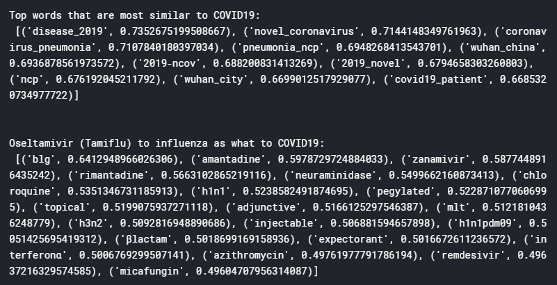
From these results, it can be seen that the word vector model has been trained pretty well, yielding terms that are quite sensible and relevant. For example, the top words that are most similar to Covid-19 includes “novel coronavirus”, “Wuhan China”, and “2019-ncov”, which are all very relevant, especially 2019-nCov which is the name of the disease before it was renamed Covid-19. The analogy case also yield interesting results, with the top ranking word “blg” stands for Chinese medicine Ban-Lan-Gan which was a popular herbal treatment for SARS. Chloroquine, a malaria treatment, as well as the drug Remdesivir, both of which been quoted to potentially effectively treat Covid-19, also appears on the list (unfortunately recent news suggests these are in fact ineffective). A bunch of antibiotics also appeared, probably referring the need to antibiotics for treating secondary infections.
So with TF-IDF and Word2Vec, we have successfully narrowed down the number of articles of interest and turn the abstracts of these articles of interest into a vector form that would allow us to perform further analysis. I have shown here that simple similarity and analogy analysis on word vectors can also yield relevant information for us to learn more about these articles. In the next blog, I will describe how cluster analysis on these word vectors can help further understand these abstracts.
References:
Stanford CS224N Lecture 2: Word2Vec Representations
Word2Vec Lecture by Jordon Boyd-Graber
Gensim Official Word2Vec Tutorial
The full notebook for the work shown here is available on Kaggle

One thought on “COVID-19 Literature Review using NLP – Part #2 TF-IDF and Word Vectors”